Average Based on Multiple Criteria

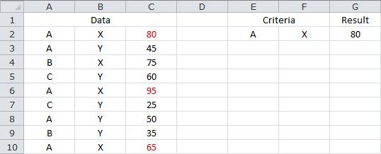
The following formula returns the average for C2:C10, where the corresponding value in A2:A10 equals the value in E2, and the corresponding value in B2:B10 equals the value in F2...
=AVERAGEIFS(C2:C10,A2:A10,E2,B2:B10,F2)
For Excel 2003 and prior versions, the following array formula can be used...
=AVERAGE(IF(A2:A10=E2,IF(B2:B10=F2,C2:C10)))
Note that the formula needs to be confirmed with CONTROL+SHIFT+ENTER. If done correctly, Excel will automatically place curly braces {...} around the formula.
Based on the sample data, the formula returns 80.
Sample Workbook: Download

